Technical notes

1. Assembling the global matrix

In the Finite Element method a dense element matrix A_el of dimensions [ndofel X ndofel] is computed for every element. Since neighboring elements share nodes, the individual element contributions need to be assembled (summed up) in the global matrix A. During the assembly every element matrix A_el is added to the global matrix A in the row/column positions determined by the node (dofs) numbers stored in the ELEMS (DOFS) arrays.

Unlike the dense element matrices the global matrix is sparse, i.e., most of its entries are zero. There is a characteristic average number of non-zero entries per row depending on the connectivity structure of the mesh. The exact number of entries per row depends on the element type and the number of degrees of freedom per node. Table 1 below gives an average number of row entries for various types of elements.

	tri3	tri6	tri7	quad4	quad9	tet4	tet10	tet15	brick8	brick27
nnz(row/col)	7	11.5	12	9	16	14.6	28.4	31.4	26.7	63

Table 1. Average number of non-zero entries in every row/column of assembled system matrix for various element types.

Since the number of entries per row of A is bounded from above by a constant, the total number of non-zero entries constitute a small (and decreasing with increasing the system size) fraction of all the matrix entries (nnz(A)~C*n vs. numel(A)=n²). Storing the zero entries and explicitly using them in computations is inefficient from the point of view of the memory and computational resources. For sparse matrices, dedicated storage formats have been developed that allow only the non-zero entries to be kept in the memory and used in computations. This is commonly done by keeping additional row and column index information along with every non-zero matrix entry.

Below we show how to use the sparse storage and how to assemble the global sparse matrix A in MATLAB.

How not to do it in MATLAB

Consider the most straightforward implementation of assembling local matrices A_el into the global matrix A for a FEM problem with one dof per node.

A = sparse(nnod,nnod);
for iel=1:nel
    indx = ELEMS(:,iel);
    ...
    %compute element stiffness matrix A_el
    ...
    A(indx,indx) = A(indx,indx) + A_el;
end

In the code fragment above the sparse matrix A initially contains only zero entries, i.e., very little memory is used by the data structure. During the execution of the element loop the sparsity pattern (the positions of the non-zero entries) of the global matrix A changes as the contributions from the elements are added. The internal data structure that holds the matrix entries and the auxiliary row/column index arrays need to be constantly reallocated and updated. In practice, in the above approach the time spent on the assembly largely exceeds the time needed to compute the element matrices.

Since the sparsity pattern is determined by the mesh, the final data structure needed to hold the sparse matrix A can be
allocated before the element loop. In this approach A explicitly stores zero entries in places (row/column pairs), which can contain non-zeros after the assembly. The matrix entries can be updated in the element loop. This requires an additional work of finding the correct memory location in the sparse data structure, but the large overhead connected with constant rebuilding of the sparse storage structure is avoided. Unfortunately, this approach is not a viable option in MATLAB for two reasons:

1. It is not possible to explicitly store zero entries in sparse matrices in MATLAB, since those are automatically removed. Thus, it is not possible to initialize an empty sparse matrix with a predetermined sparsity pattern.
2. In our experience updating a small set of entries of a sparse matrix in MATLAB also involves a substantial overhead. This could be caused by the additional time MATLAB spends on verifying that a sparse matrix only contains non-zero entries, which requires reading all the matrix entries from the memory – an overhead that grows with the system size.

Overcoming the two deficiencies would require a major modification of the MATLAB sparse class.

Triplet sparse storage

A workaround solution is to compute and store all the element matrices A_el first and assemble them in one call to MATLAB sparse function, as shown in the code fragment below.

A_all = zeros(nnodel*nnodel,nel);
for iel=1:nel    
    ...
    %compute element stiffness matrix A_el
    ...
    A_all(:,iel) = A_all(:,iel) + A_el(:);
end
 
indx_j = repmat(1:nnodel,nnodel,1); 
indx_i = indx_j';
Ai = ELEMS(indx_i(:),:);
Aj = ELEMS(indx_j(:),:);
 
A = sparse(Ai,Aj,A_all);

In this approach all the element matrices are first stored in A_all array. Next, the row and column indices for every entry of all the element matrices are computed (Ai, Aj). This method of representing a sparse matrix is called the triplet format: for every matrix entry the corresponding row/column information is stored explicitly. Duplicate Ai, Aj pairs exist in the triplet list. The global matrix assembly is performed in one call to a dedicated MATLAB function sparse, which adds the duplicate entries.

This implementation is much faster than the first described approach. The disadvantages are that all the element matrices need to be stored in the A_all array prior to the assembly. The memory requirements are additionally increased due to the need to store the arrays containing row/column indices. Due to the duplicates the number of entries in the triplet storage can vary between 6.3 to 1.4 times the number of non-zero entries in the assembled global matrix A. The exact amount of memory overhead depends on the element type (see the Table 2). If the matrix assembly is not followed by the much more memory intensive Cholesky factorization, the elevated memory requirements related to the (Ai, Aj, A_all) arrays might restrict the problem size that can be solved.

element type	tri3	tri6	tri7	quad4	quad9	tet4	tet10	tet15	brick8	brick27
ratio (triplet/crs)	2.6	1.6	1.4	1.8	1.3	6.3	2.6	1.6	2.4	1.4

Table 2. Ratio of the number of entries in the triplet to assembled sparse matrix format.

In the triplet sparse format every non-zero matrix entry requires three data values: A_all – the value of the entry, and Ai/Aj – row and column index of the entry. The MATLAB function sparse only takes as arguments A_all/Ai/Aj of type double. This means that in this storage format every triplet requires 3*8=24 bytes of memory. sparse removes the duplicate triplets and converts the matrix into MATLAB native sparse format CCS (Compressed Column Storage). In CCS sparse matrix A is stored column by column and every non-zero entry only requires its row index in addition to the value. In MATLAB Both row indices and data values use 8 bytes of memory per non-zero entry. Hence, the memory requirements for the assembled matrix A are 1.5 times the duplicates ratio lower than for the triplet storage.

The algorithmic complexity of converting the triplet sparse format to the native MATLAB sparse format (CCS – Compressed Column Storage) is O(n), i.e., it is linear with the system size n. It means that this approach is scalable with the number of elements and nodes in the mesh – doubling the mesh size requires twice the number of operations and double the amount of memory to assemble the global matrix A.

sparse vs. sparse2

The efficiency of the triplet approach can be further improved by using the sparse2 function provided by the SuiteSparse package from Tim Davis [1]. The entire procedure of global matrix assembly is essentially the same as described above, with minor differences that result in significant execution time improvement

1. Ai and Aj index arrays must be of type double in the case of MATLAB sparse routine. For sparse2 they can be of type int32. Since doubles use 8 bytes and integers use 4 bytes, less memory is required.
2. Since accessing memory takes time, using integers for the Ai/Aj index arrays speeds up the code.
3. sparse2 supports creation of logical sparse matrices, i.e., matrices that contain 1 where there is a non-zero entry. In this case the matrix entries are also stored as integers instead of doubles, which further speeds up the code. Logical matrices can be used e.g., to compute the reordering.

sparse_create

In the triplet approach shown in the code fragment above the index arrays Ai/Aj are explicitly constructed based on the element dof information by generating all-to-all connections for all the dofs. However, explicit construction of Ai/Aj index arrays is not necessary and the index pairs for every element matrix stored in A_all can be generated on the fly from ELEMS by a sparse-like routine.

sparse_create is a MEX function distributed with MILAMIN that takes as the parameters the ELEMS and A_all arrays and assembles the global system matrix A. It can create symmetric (lower triangular part) and general matrices

A = sparse_create(ELEMS, A_all, 0);   % general sparse matrix
A = sparse_create(ELEMS, A_all, 1);   % symmetric sparse matrix, lower triangular part

The memory requirements of sparse_create are significantly smaller than of the approach using triplet storage. Except for the A_all, it does not require any space to be allocated for the duplicate entries. This results in significant memory savings for the ‘lighter’ elements like tri3 and tet4 (see Table 2). Thanks to much smaller memory requirements it is usually as fast as or faster than sparse2. In addition, it does not require the Ai/Aj index arrays to be created, which saves even more time.

Instead of A_all one can supply no arguments or ‘true’, in which case a symbolic sparse matrix is created containing 1 in all the non-zero entries. This syntax is useful when the matrix is only needed to compute reordering of the nodes.

A = sparse_create(ELEMS);

Algorithmic complexity of sparse_create is also O(n).

Efficiency tests

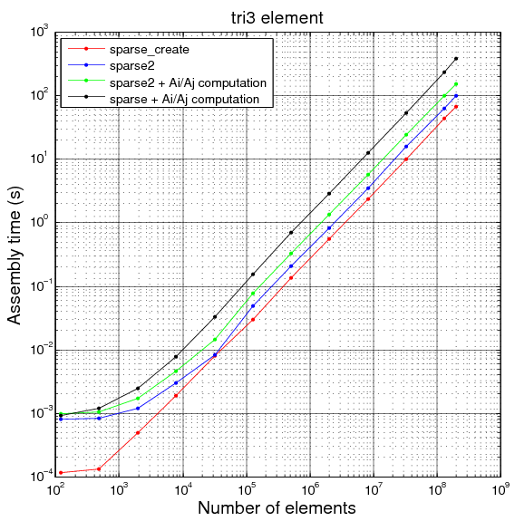
Figure 1. Time required to perform global sparse matrix assembly for 2D meshes of 3-node triangular elements using different methods. Symmetric sparse matrix is created. Computer: valinor.

Figure 1 shows the time needed to assemble the lower triangular part of the global sparse matrix A given the element matrices A_all using the described methods. The 3-node triangular element meshes are considered. For this element type sparse_create is clearly better than the approach based on the triplet storage, especially if the time required to compute the Ai/Aj index arrays is included.

	tri3	tri6	tri7	quad4	quad9	tet4	tet10	tet15	brick8	brick27
sparse_create	2.98	0.63	0.46	3.30	0.53	2.57	0.24	0.08	0.86	0.04
sparse2	2.0	0.39	0.28	1.35	0.28	0.96	0.17	0.07	0.37	0.03
sparse	0.52	0.16	0.12	0.41	0.07	0.34	0.07	0.03	0.12	0.01

Table 3. Efficiency in millions of elements per second of the different methods to assemble the global matrix A Time needed to compute Ai/Aj index arrays is included in results of sparse2 and sparse. Computer: valinor.

The performance gain of sparse_create in Figure 1 is due to a relatively high number of duplicate entries for this type of mesh, as shown in Table 2. For other element types the advantage of sparse_create in terms of execution time might be lower, as shown in the Table 3.

The memory requirements of the different implementations are shown in Table 4.

	sparse_create	sparse2	sparse
A_elem	1.6	1.6	1.6
ELEMS	0.4	0.4	0.4
NODES	0.3	0.3	0.3
A	1.2	1.2	1.2
Ai + Aj	0	1.6	3.2
assembly workspace including Ai/Aj	3.1	9.5	10.9
maximum amount of memory allocated at any time	5.4	11.8	13.2
assembly time (s)	10	25	56

Table 4. Memory usage (in GB) of different global matrix assembly implementations. 3-node triangular element, 33 million elements, 16.5 million nodes.

2. System solution

The approximate solution to the original PDE is obtained by solving a linear system of equations

A*x = b

where A is a square coefficients matrix of size n*n (system matrix), x is the solution vector of size n, and b is the right-hand side vector of size n. The solution vector x could be obtained by a direct computation of the inverse of the matrix A as

x = A^-1*b

However, this approach is not practical. The matrix A is sparse, i.e., the fraction of non-zero entries is low. On the other hand, the inverse matrix A^-1 is a dense matrix even for the simplest tri-diagonal system of equations. Hence, the large memory requirements severely limit the systems that can be solved in practice. A system of 1 million degrees of freedom (unknowns) would require around 8 terabytes of RAM to store the inverse matrix (1e6^2*8).

There are numerous efficient algorithms that limit the number of arithmetic instructions and bytes of memory required to solve sparse systems of linear equations on modern computers. Possibly the most basic algorithm is the LU factorization – a variant of the Gaussian elimination. The system matrix A is represented as a product of two matrices L and U

A = L*U

such that L is a lower-triangular matrix, and U is an upper-triangular matrix. The original system of equations is now expressed as

(L*U)*x = b

and the solution vector x can be obtained by

x = U^-1*(L^-1*b)

Since the LU factors are triangular, the solution vector can be easily obtained by forward and backward substitution instead of explicitly computing the inverse matrices. Using the MATLAB notation we write

x = U\(L\b)

where the backslash operator (\) denotes the forward/backward substitution.

Compared to the naive approach of computing A^-1, sparse factorization can only perform better if the LU factors are sparse. MILAMIN renumbers the unknowns and the matrix to minimize the number of non-zero entries in the factor using various fill-reducing reordering techniques. Essentially, the unknowns are renumbered and the matrix is permuted using a permutation vector

perm = f(A)

A = A(perm,perm)

Further savings on memory and operation requirements can be made for special types of matrices. For example, symmetric positive definite matrices can be factorized using the Cholesky factorization

A = L*L'

where L is a lower triangular factor and L’ is its transpose. Computing only one lower triangular factor roughly halves the number of operations and the amount of memory required.

In short, the algorithm for the solution of the global system of linear equations used in MILAMIN consists of four major steps:

• Application of the boundary conditions to A
• Reordering of the unknowns to reduce the number of non-zero entries in the factor (A=A(perm,perm))
• Factorization of the reordered system matrix (A=L*L’)
• Solution of the factorized system using backward-forward substitution (x = L\(L’\b))

We present several approaches to perform the above steps using MATLAB and the MILAMIN software package. Our major interest is the efficiency of the implementation, and the memory consumption. We show how to solve large systems in a reasonable time on modern multi-core shared memory CPU architectures.

2.1 Boundary conditions

Consider the linear system of equations

A*x = b

where A is a symmetric matrix discretizing a scalar-valued elliptic PDE (A is a discrete Laplace operator). Finding solutions to elliptic PDEs on finite domains requires setting boundary conditions e.g., the Dirichlet, Neumann, or periodic.

We consider efficient application of the Dirichlet boundary conditions, i.e., the x value in the boundary nodes is explicitly defined. Assume node with index k is a boundary node. To set the value of x(k)=1 the k‘th row of the system matrix A is modified in the following way

A(k,i)=0 for i=1:n and i!=k
A(k,k)=1

In other words, the diagonal entry of the k‘th row is set to one, and all other entries are set to 0. The k‘th entry of the right-hand side vector b is set to 1

b(k)=1

This way the k‘th equation is trivial and reads

1*x(k)=1

Note that after this modification the system matrix A is no longer symmetric. The non-zero columns of the k‘th matrix row have been explicitly set to 0. The symmetry can be regained by setting all the rows in the k‘th matrix column to 0. This is done by eliminating the known x(k) from all the equations it is part of. For every equation i, for which A(i, k) is non-zero the right-hand side vector entry b(k) is modified as

b(k) = b(k) - A(i,k)*x(k)

and the system matrix is modified as

A(i,k) = 0

In general, there are in total n degrees of freedom. Assume there is a set of Dirichlet boundary nodes with indices Bc_ind and boundary values x(Bc_ind) = Bc_val. We denote the indices of the unconstrained nodes as Free_ind. The boundary conditions can be implemented by directly applying the above described modifications to A and b for every boundary node separately.

Free_ind = 1:n;
Free_ind(Bc_ind) = [];
 
% for all boundary nodes
for id=1:length(Bc_ind)
 
    % deal with equation k
    k = Bc_ind(id);
 
    % eliminate the k'th variable
    rows = A(Free_ind,k);
    b(Free_ind) = b(Free_ind) - rows*Bc_val(id);
 
    % modify A and b
    A(:,k) = 0;
    A(k,:) = 0;
    A(k,k) = 1;
    b(k) = Bc_val(id);
end

This implementation is very inefficient since every boundary node is processed independently. In particular, resetting row (and column) entries of a sparse matrix to zero introduces costly changes to the sparsity pattern. Avoiding multiple modifications of the sparsity pattern of A is expected to minimize the related overhead.

The code fragment below presents two different approaches to apply the Dirichlet boundary conditions in MATLAB efficiently. Instead of modifying matrix entries, the rows and columns corresponding to the boundary nodes can be all together removed from the system. The update to the right hand side vector is recast into a (dense) matrix-vector multiplication. For symmetric matrices only the upper- or lower-triangular part of A needs to be stored and the implementation is modified accordingly.

 Free = 1:n;
 Free(Bc_ind) = [];
 b = zeros(n,1);
 b(Bc_ind) = Bc_val;
 
% Approach Ia:
 b = b - (A(:,Bc_ind) + cs_transpose(A(Bc_ind,:)))*Bc_val';
% Approach Ib:
 b = b - (A(:,Bc_ind) + (A(Bc_ind,:))')*Bc_val';
% Approach IIa:
 b = b - A*x - (x'*A)';
% Approach IIb:
 b = b - A*x - A'*x;
 
% Elimination of trivial equations 1
 A = A(Free_ind,Free_ind);
 
% Elimination of trivial equations 2
 A(:,Bc_ind) = [];
 A(Bc_ind,:) = [];

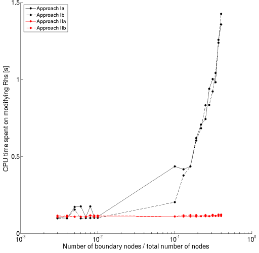
Execution time of the above implementations on an example desktop architecture is compared in Figure 2 below. The system size is approximately one million degrees of freedom. The number of Bc_ind nodes in the system varies. When the fraction of the boundary nodes is smaller than 1% we observe no substantial difference in the performance of the four methods (Ia,Ib,IIa,IIb) to modify the right-hand side vector b. Most practical two-dimensional models are in this regime. For higher fractions of up to 40% the approaches IIa and IIb perform equally well as for the lower fractions. Implementations Ia and Ib are significantly less efficient in this regime.

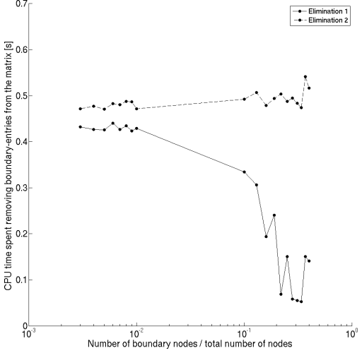
Figure 3 below presents the execution time of the two studied methods to eliminate the rows and columns corresponding to the boundary nodes from the system matrix A. When the fraction of the boundary nodes is smaller than 1% the Elimination 1 is slightly more efficient than Elimination 2. For higher fractions of boundary nodes Elimination 1 becomes increasingly more efficient, while the performance of Elimination 2 remains unchanged.

In summary, approaches IIa or IIb should be used to modify the right-hand side vector b, and Elimination 1 should be used to remove the trivial equations for the boundary nodes Bc_ind from the system matrix A.

2.2 Reordering

Direct solvers of linear systems of equations factorize the system matrix A into a product of lower- and upper-triangular matrices, e.g. A=L*U in case of LU factorization, or A=L*L^T in case of Cholesky factorization. Although for the problems considered here the system matrix A is sparse (nnz(A) << n²), usually the number of non-zero entries in the factors is significantly larger than in the system matrix. New non-zero entries are added in the factors compared to the system matrix A and in the worst case scenario the factors can be dense triangular matrices.

The number of the additional non-zero entries introduced during the factorization, often referred to as the fill-in, depends on the structure of A. Renumbering of the unknowns prior to the factorization alters the non-zero structure (the sparsity pattern) of A and therefore affects the fill-in. The aim of the reordering step is to find a permutation of the unknowns that minimizes the fill-in. To summarize, the fill-reducing reordering is crucial since it decreases both memory and computational requirements:

• The fill-in determines the amount of memory required to store the factors. If the memory requirements are larger than the available RAM the factorization will either fail, or will be significantly slower due to swapping.
• The amount of fill-in affects the flop count, and consequently the computational time required to perform the factorization.
• The number of non-zero entries in the factors affects the flop count and the computational time required to perform the backward and forward substitution.

Finding the optimal reordering that would result in a minimum fill-in is an NP-hard problem. Essentially, this means that for a general sparse matrix there is no efficient algorithm to find the best permutation and effectively all of the permutations need to be checked. Clearly, this is not practical even for systems with hundred unknowns. Various heuristic reordering techniques have been developed that aim at decreasing the fill-in during sparse factorization well enough and in a reasonable time. In this section we present a comparison of the AMD and METIS algorithms. AMD (Approximate Minimum Degree) is an built-in MATLAB routine, while METIS is accessible in MATLAB through the SuiteSparse package. These techniques are very effective for matrices resulting from discretization of PDEs using local methods.

Reordering, Fill-in, and Flop Count during factorization

Figure 4 presents a comparison of the effectiveness of AMD and METIS reorderings. The number of non-zero entries in the factor nnz(L) is shown as a function of the system size for 2D and 3D domains discretized with 3-node triangles and 4-node tetrahedrons, respectively. In the log-log space nnz(L) can be fitted by a linear function of the number of mesh nodes n. This means that nnz(L) is a power-law function of n

nnz(L) = n^α

The larger the exponent α, the faster the number of non-zero entries in the factor grows with the system size. In practice this means that lower exponents allow larger systems to be solved on a computer with a given memory configuration. In the shown comparison the exponent is larger for AMD reordering in both 2D and 3D: 1.19 and 1.59, respectively, compared to 1.13 and 1.42 obtained using METIS.

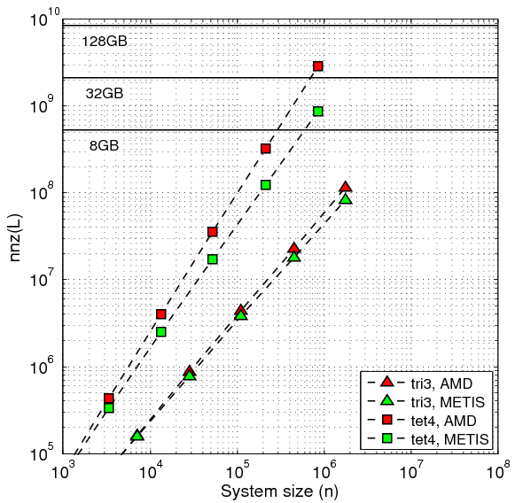
Figure 4. Number of non-zero entries in the factor for AMD and METIS reorderings. Matrices resulting from FEM meshes with 2D 3-node triangular elements and 3D 4-node tetrahedral elements. One degree of freedom per mesh node.

Figure 5 presents nnz(L) as a function of the system size n for two- and three-dimensional meshes and for various elements. Only METIS reordering is shown. Sparse matrices considered result from Finite Element discretization of the Poisson’s equation (1 degree of freedom per mesh node). The power-law exponent is different in two and three dimensions, but similar for different element types.

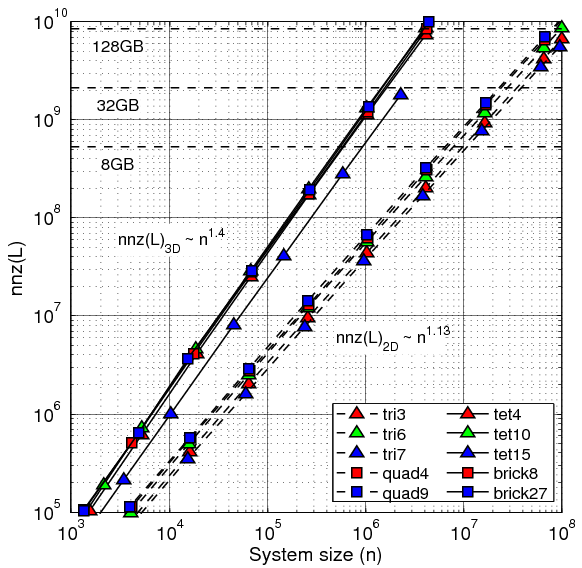
Figure 5. Number of non-zero entries in the factor depending on spatial dimension of the mesh, system size and element type. One degree of freedom per mesh node. METIS fill-reducing reordering. Memory requirements for the factors assuming MATLAB sparse storage marked for reference.

Figure 6 presents the number of floating point operations (flop count) required to perform the factorization of the global stiffness matrix after reordering. Also in this case the number of flops required is a power-law function of the system size. The table below summarizes the power-law exponents for matrices resulting from 2D and 3D problems averaged for different element types.

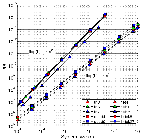
Figure 6. Flop count of the Cholesky factorization depending on spatial dimension of the mesh, system size and element type. One degree of freedom per mesh node. METIS fill-reducing reordering.

	2D		3D
	nnz(L)	flop count	nnz(L)	flop count
AMD
METIS	1.13	1.56	1.40	2.06
Theoretical bounds	n log(n)	1.50	1.33	2.00

 

A system size of one million nodes

As seen in Figure 4, for systems with around 1 million nodes in 2D the difference in memory consumption is not very signifficant. The memory usage due to the factor is 1.7 GB and 1.2 GB for AMD and METIS reorderings, respectively. The difference shows much more in 3D: with AMD the factor uses 43 GB of RAM, while with METIS only 13 GB.

For a system size of one million degrees of freedom in 2D the number of non-zero entries in the factor resulting from the METIS reordering is approximately two times lower than that obtained using AMD. The difference is approximately five times for the 3D problems. Considering the flop count, for 2D and 3D problems METIS results in 2 times and 15 times less work, respectively.

CPU Time Required to Compute Reordering

The reordering step is itself a rather costly operation. The time required to find the permutation of the unknowns should be considered in view of the number of times the permutation vectors can be reused. Note that the permutation only needs to be computed when the mesh topology changes. Hence, whether a best possible reordering is crucial, or whether the reordering time also contributes significantly to the total solution time depends on the problem at hand.

Figure 4 above shows the CPU time required to find the reordering using AMD and METIS. Reordering is computed using sparse matrices resulting from two-dimensional meshes of 7-node triangular elements, one degree of freedom per node. Note that the CPU time spent on the reordering scales non-linearly with the system size, with power-law exponents varying from 1.06 – 1.16 for both reordering schemes. AMD appears to be generally more efficient than METIS, with approximately 6 times shorter CPU times for all system sizes.

Summary of the Comparison of AMD and METIS Reordering Schemes

We have presented the results from three different studies, in which we compared the performance of the AMD and METIS reordering schemes. While it takes less CPU time to compute the reordering using AMD scheme, it results in a larger number of operations (nop) required to perform the Cholesky factorization, as well as higher fill-in (nnz) of the matrix. The benefit from using METIS, in terms of nop and nnz, is higher for larger system sizes, as a result of super-linear scaling, and is especially significant for the three-dimensional problems. If the reordering can be reused for a large number of steps, it is recommended to use the METIS scheme.

Application of the Reordering to the Global System of Linear Equations

In this subsection we discuss two different approaches to apply the computed permutation vectors to the global stiffness matrix, only the lower part of which is stored. First approach is presented in Code Fragment 1, and utilizes the external libraries cs_transpose and cs_symperm, provided by the Suite Sparse package. The second approach is presented in Code Fragment 2, and only utilizes the inbuilt MATLAB-routines. The computational time required to carry out each of these code fragments, as a function of system size, is presented in the figure below. We observe that the Code Fragment 2 is more efficient, with an increasing gain for larger system sizes.

Code Fragment 1:

 A = cs_transpose(A);
 A = cs_symperm(A,perm);
 A = cs_transpose(A);

Code Fragment 2:

 A = A(perm,perm);
 A = tril(A) + triu(A,1)';

2.3 Cholesky factorization

In the cases when the system matrix A is symmetric positive definite (SPD) the Cholesky factorization can be used to decompose the system matrix A into a product of two triangular matrices

A = L*L'

where L is a lower triangular factor and L’ is its transpose. Whenever applicable, the Cholesky algorithm is advantageous to other direct methods of solving linear systems of equations.

1. Only the lower triangular part of matrix A needs to be computed and assembled in the memory.
2. The Cholesky algorithm only computes the lower triangular factor, which roughly halves the number of operations and the amount of memory required.
3. Cholesky factorization is fully deterministic and does not depend on the matrix entries, i.e., it does not require pivoting. Consequently, symbolic factorization can be used to determine the exact non-zero structure of the factor based on the non-zero structure of A before the actual factorization is computed. This improves the performance significantly because required memory structures can be pre-allocated beforehand.

MATLAB is distributed with CHOLMOD, a fast Cholesky algorithm implementation by Tim Davis [1]. Factorization of a symmetric sparse matrix A, of which only the lower triangular part is stored in the memory, is invoked with the following syntax

L = chol(A,'lower');

Remark: For MATLAB versions older than 2011a it is recommended to download the newest version of CHOLMOD directly and compile it to have a better performing Cholesky solver. MILAMIN2 will attempt to do this automatically.

Sequential Factorization Performance

The time required to compute the factor is determined by two major factors: the system size n, which determines the factorization operation count, and the computational capabilities of the computer. As shown in the Reordering section, using METIS reordering the number of FLOPs required to compute the factor is proportional to n^1.56 and n^2.06 for 2D and 3D problems, respectively.

2D Problems

Assuming the computer used to perform the calculations has a performance of X floating point operations per second (FLOP/s), the time required to factorize a matrix for a 2D thermal problem can be estimated as

t_2D(n) = C * n^1.56 / X

where C depends on the element type used and the number of degrees of freedom per node. In practice the above performance model is modified by the fact that the computational performance during factorization also depends on the system size n, i.e., X=X(n), see Figure 7.

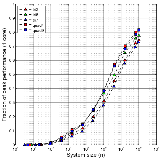
Figure 7. Efficiency on 1 CPU core (or fraction of peak FLOP/s performance) of Cholesky factorization for matrices resulting from 2D thermal problems discretized using a variety of elements. The computer used in the tests was Valinor - a Dell server with Xeon E7- 4870 CPUs (see Tested Computer Architectures section). Peak per-core performance of 11.2 GFLOP/s.

One conclusion that can be drawn from this figure is that the CPU can compute the factorization more efficiently for larger matrices. There are a number of reasons for this behavior.

1. The performance of Cholesky factorization largely depends on the performance of BLAS Level 3 dense matrix-matrix multiplication (GEMM) and triangular solve with multiple right-hand sides (TRSM) implementations. On modern multi-core CPU architectures BLAS L3 is often advertised to run close to (more than 90%) the peak multi-core performance for large enough matrices. However, for small matrices the performance is well below the peak of even a single CPU core. Thus, performance of the Cholesky solver depends on the types of dense matrices being multiplied. (Note that in tests presented in Figure 7. we used a single-threaded BLAS. Parallel performance is considered later.)
2. During sparse Cholesky factorization BLAS L3 routines are executed for a variety of dense matrices with different dimensions. In the Reordering section it has been demonstrated that the number of non-zeros in the factor grows like system size n to some power greater than 1. In fact, it can be observed that for the growing system size n the dimensions of the matrices that need to be multiplied also grow. For large enough n BLAS L3 calls for the largest matrices start to dominate the total execution time, hence the improved overall efficiency of Cholesky factorization.
3. For larger systems the overhead connected with initialization of the Cholesky algorithm is relatively smaller. In the symbolic factorization stage the number of non-zero entries in every row of the factor is computed. The complexity of symbolic factorization is linear with respect to the system size. Hence, the overhead introduced by this stage disappears with the system size.

Figure 7 demonstrates that for 2D thermal problems the factorization achieves only around 50% of the peak CPU performance for systems as large as 4 million degrees of freedom. 70-80% of the peak is achieved for systems with roughly 100 million degrees of freedom. Note that the performance is better for quad elements and the 6-node triangular element, while lower performance is observed for the 3- and 7-node elements.

3D Problems

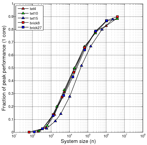
Figure 8. Efficiency on 1 CPU core (or fraction of peak FLOP/s performance) of Cholesky factorization for matrices resulting from 3D thermal problems discretized using a variety of elements. The computer used in the tests was Valinor - a Dell server with Xeon E7- 4870 CPUs (see Tested Computer Architectures section). Peak per-core performance of 11.2 GFLOP/s.

Figure 8 shows factorization efficiency results for 3D thermal problems and various element types. Clearly, factorization efficiency for 3D problems is significantly better than for 2D. On the tested computer 50% of peak FLOP/s performance is achieved for problems with approximately 10⁴ mesh nodes. For models with approximately 3-4 million nodes the solver runs at over 10 GFLOP/s, around 90% of a single core peak performance.

Parallel Factorization Performance

The literature on parallel direct solvers for various types of linear systems of equations is vast. Obtaining a scalable and highly parallel direct solver implementation is quite challenging considering both the technical requirements and the complexity of the algorithms. The approach used in MATLAB can be implemented relatively easily on multi-core systems with shared memory. It is based on the observation that the Cholesky solver makes extensive use of the BLAS library, especially of the GEMM/TRSM implementations. Hence, even though the CHOLMOD solver used by MATLAB is sequential, it can be parallelized to some extent by providing a parallel BLAS implementation.

2D Problems

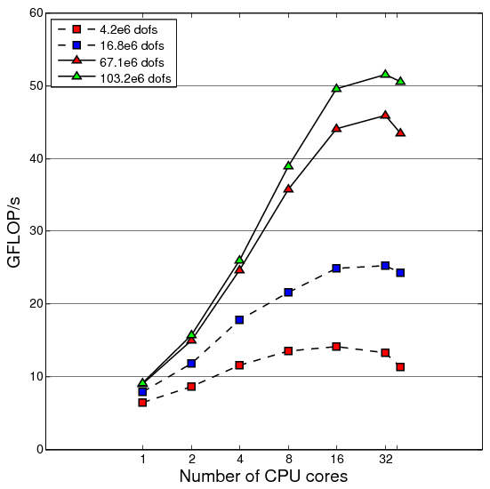
Figure 9. Parallel factorization performance, 2D thermal problem, 4-node quad element.

Figure 9 presents the parallel performance of the Cholesky solver for a chosen 2D element on the 40-core Valinor SMP server. The peak performance of a single core on this computer is 11.2 GFLOP/s. For the largest studied system size (100 million dofs) the observed single core performance is roughly 9 GFLOP/s, 80% of peak (compare this to single core efficiency shown in Figure 7). Increasing the number of cores up to 16 results in some speedup. Further increase in the number of cores is ineffective or even degrades the performance. Similar behavior is observed for the smaller system sizes.

For the largest problem size the highest achieved performance of ~50 GFLOP/s is more than 5 times the single core performance. Considering that 16 cores were used to achieve the 5 times speedup it is clear that the per-core efficiency significantly degrades in the parallel run. Indeed, 16 cores have a peak performance of 16*11.2=179.2 GFLOP/s. Hence, the observed 50 GFLOP/s corresponds to around 28% of the theoretical peak, while the single-core efficiency was 80%.

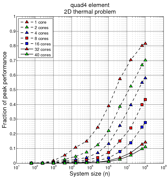
Figure 10. Efficiency (fraction of peak multi-core performance) of parallel Cholesky factorization. Matrices resulting from 2D meshes using quad4 elements. Valinor server.

Figure 10 shows a systematic study of the efficiency of the parallel factorization for many 2D problem sizes and the 4-node quad element. Factorization efficiency defined as the fraction of the peak FLOP/s performance is shown for different number of CPU cores. For every parallel configuration the peak performance is calculated taking into account the number of cores actually used.

As also seen in Figure 7, the single core factorization efficiency increases with the system size reaching 80% for the largest studied systems. Figure 10 demonstrates that when factorizing a given system of equations using an increasing number of cores the efficiency quickly degrades. However, as in the sequential case, for a fixed number of cores the efficiency clearly increases with an increasing system size. One can now ask how fast does the system size n need to grow to assure the same factorization efficiency on increasing number of cores. For example, in the considered 2D case 50% efficiency is obtained on 1 core for a problem size of roughly 2*10⁶ nodes. What is the problem size for which the Cholesky solver will run with 50% efficiency on 2 cores? Such relation between the problem size n and the number of cores is called isoefficiency function.

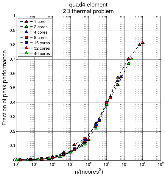
Figure 11. Efficiency of parallel Cholesky factorization as a function of the system size scaled by the number of CPU cores squared. Matrices resulting from 2D meshes using quad4 elements. Valinor server.

Figure 11 presents the same performance results as Figure 10, but the X axis – the problem size n – is in this case scaled by the number of cores squared. All the lines for parallel configurations with different number of CPU cores plot on the same curve. This means that with the employed parallelization technique, for the studied architecture, and for the 2D thermal problems discretized using 4-node quad element

E = f(n/(ncores²))

where E denotes efficiency. The above relation also holds for other tested 2D elements. Since for the single core case ncores²=1 and hence E=f(n), Figure 7 in fact shows the isoefficiency functions for different 2D element types. The usefulness of the above considerations can be demonstrated by the following practical examples.

Example 1. Assuming we want to use the 32 cores on Valinor with 50% efficiency to solve a 2D thermal problem, what is the system size n required? From Figure 11 we see that for 50% efficiency

n/ncores² = 2*10⁶

Hence, if we use ncores=32

n = 2*10⁶*32² = 2*10⁹

Example 2. How much time will it take to factorize a system of size n=10⁸ dofs using 32 CPU cores assuming METIS reordering is used?

n/ncores² = 10⁸/32² = 10⁵

From Figure 11 we read that the expected factorization efficiency is in this case 18%. Hence, the expected factorization performance is roughly 0.18*32*11.2 = 64 GFLOP/s. From Figure 12 in the Reordering section we can infer that factorization of the given system will require around 5*10¹³ floating point operations. Hence, with the expected performance it will take roughly

t = 5*10¹³ [FLOP] / 64*10⁹ [FLOP/s] = 781 [s]

The actual measured performance for the 4-node quad element and a system with 103 million dofs is 52 GFLOP/s and the factorization time on 32 CPU cores was 847 seconds.

3D Problems

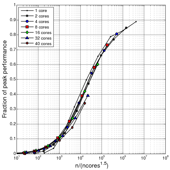
Figure 12. Efficiency of parallel Cholesky factorization as a function of the system size scaled by the number of CPU cores in 1.5 power. Matrices resulting from 3D meshes using tet4 elements. Valinor server.

Figure 12 shows the isoefficiency function for the 4-node tetrahedral element. Parallel Cholesky solver is more scalable in 3D since in order to keep constant efficiency the problem needs to grow slower with the system size than in the 2D case

E = f(n/(ncores^1.5))

or the system size needs to grow with the number of processors in power 1.5. These results are in agreement with other studies found in the literature on massively parallel sparse factorization [2].

Clearly, sparse factorization for 3D problems is both more efficient for smaller system sizes, and more amenable to parallelization than in the 2D case. However, as shown in the Reordering section, the operation count and the number of non-zero entries in the factor grows much faster for 3D problems.

Example 3. In Example 2. above we considered a 2D problem with 10⁸ nodes. In this case factorization required approximately 10¹⁴ operations. For 3D problems similar number of operations is needed already for problems of size n=3*10⁶. Using 32 CPU cores to factorize this problem yields

n/ncores^1.5 = 3*10⁶/(32^1.5) = 2*10⁵

From Figure 12 we can see that in this case the expected factorization efficiency is around 75%, i.e., 265 GFLOP/s. This is more than 4 times faster than in the corresponding 2D case. However, in terms of the number of mesh nodes the 3D problem is 35 times smaller than its 2D counterpart. Consequently, in this example the 3D models are roughly 9 times more expensive per grid node.

References

• [1] T. Davis, SuiteSparse, http://www.cise.ufl.edu/research/sparse/SuiteSparse/
• [2] A. Gupta, S. Koric, T. George, Sparse Matrix Factorization on Massively Parallel Computers, IBM Research Report, 2009

2.4 Forward and backward substitution

Once the system matrix A has been factorized using the Cholesky factorization the original linear system of equations can be represented as

LL^Tx_perm = b_perm

Note that the x and b vectors are permuted using the fill-reducing reordering used. The permuted solution vector x_perm is obtained using forward substitution

L^Tx_perm = L^-1b_perm

followed by backward substitution

x_perm = (L^T)^-1L^-1b_perm

Using MATLAB the above can be implemented as

Code Fragment 1:

x(Free_ind(perm)) = L'\(L\b(Free_ind(perm)));

where perm is the permutation vector and Free_ind is a vector holding the indices of unconstrained nodes (see the Boundary Conditions section).

Since the same number of floating point operations needs to be performed in the forward (L\) and backward (L’\) substitutions, in the ideal scenario each step should take the same amount of time. However, in the above implementation the factor L needs to be explicitly transposed in order to perform backward substitution. The additional work causes this implementation to be sub-optimal.

One option is to implement the above using the ‘/’ (or mrdivide MATLAB function). This avoids explicit computation of L’, i.e., only L is used in the MATLAB code:

Code Fragment 2:

x(Free_ind(perm)) = (L\b(Free_ind(perm)))'/L;

However, according to the documentation mrdivide performs the transposition of the matrix internally:

 /   Slash or right matrix divide.
    A/B is the matrix division of B into A, which is roughly the
    same as A*INV(B) , except it is computed in a different way.
    More precisely, A/B = (B'\A')'. See MLDIVIDE for details.

Effectively, both above implementations have the same performance.

The performance of backward substitution can be significantly improved with the help of the external library SuiteSparse. The function cs_ltsolve uses the lower-triangular factor L and performs the backward substitution without explicit matrix transposition

Code Fragment 3:

x(Free_ind(perm)) = cs_ltsolve(L,cs_lsolve(L,b(Free_ind(perm))));

As seen in Figure 13, this has a major impact on performance. Using SuiteSparse to perform both the forward and backward substitution improves the performance roughly four times over a native MATLAB implementation. The red curve shows the time needed to perform the native MATLAB forward substitution (L\) only. It takes roughly half the time needed by the SuiteSparse implementation to compute both substitution steps, which agrees with our expectations that the two stages should take the same time. The blue curve shows the time taken by the native MATLAB backward substitution (L’\). Clearly, the speedup of SuiteSparse comes from avoiding the explicit transposition of the factor.

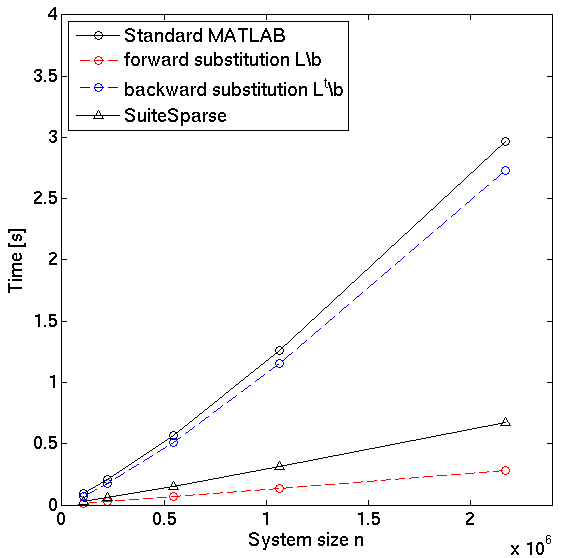
Figure 13. Performance of forward and backward substitution using native MATLAB and SuiteSparse implementations.

3. Tested computer architectures

The performance results presented throughout this website have been obtained using the following computers

Name	Model Name	CPU GHz	Num. CPUs	Num. CPU cores	Operating System	MATLAB-version
Valinor	Intel(R) Xeon(R) CPU E7- 4870 @ 2.40GHz	2.4 (2.8)	4	10	Red Hat Enterprise Linux Server release 6.1 (Santiago)
Hemlokk	Intel(R) Xeon(R) CPU E5530 @ 2.40GHz	2.4 (2.66)		4	Red Hat Enterprise Linux Client release 5.7 (Tikanga)
Palme	Intel(R) Xeon(R) CPU X5472 @ 3.00GHz	2.3		4	Linux 2.6.18-238.5.1.el5
Kauri	Dual-Core AMD Opteron(tm) Processor 2220	2.8	2	2	Red Hat Enterprise Linux Client release 5.7 (Tikanga)
Seder	Intel(R) Core(TM)2 Quad CPU Q9550 @ 2.83GHz	2.8		4	Linux 2.6.18-238.12.1.el5

System specifics of all the computers used to investigate the performance of MILAMIN